MLLab[1]: Linear Regression
Basic Data Operate
1
2
3
4
5
6
7
8
| %pip install seaborn
import pandas as pd
import numpy as np
import matplotlib.pyplot as plt
import seaborn as sns
sns.set(context="notebook", style="whitegrid", palette="deep")
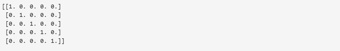
A=np.eye(5)
print(A)
|
Output:
1
2
3
4
5
6
7
| df = pd.read_csv('ex1data1.txt',names=['人口','利润'])
df.head()
df.info()
|
Output:)

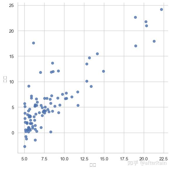
Data Visualize
computeCost
1
2
3
4
5
6
7
8
9
10
11
| def computeCost(X,y,theta):
inner=np.power((X*theta-y),2)
return np.sum(inner)/(2*len(X))
df.insert(0,'ONE',1)
cols = df.shape[1]
X = df.iloc[:,0:cols-1]
y = df.iloc[:,cols-1:cols]
X = np.matrix(X.values)
y = np.matrix(y.values)
theta = np.matrix(np.array([0,0]
computeCost (X,y,theta)))
|
Output:np.float64(32.072733877455676)
gradientDescent
1
2
3
4
5
6
7
8
9
10
11
12
13
14
15
16
17
18
19
20
21
22
23
24
| def gradientDescent(X,y,theta,alpha,iters):
temp=np.matrix(np.zeros(theta.shape))
parameters= int(theta.ravel().shape[1])
cost=np.zeros(iters)
for i in range(iters):
error=(X*theta.T)-y
for j in range(parameters):
term = np.multiply(error, X[:,j])
temp[0,j] = theta[0,j] - ((alpha / len(X)) * np.sum(term))
theta=temp
cost[i] = computeCost(X,y,theta)
return theta,cost
alpha=0.01
iters=1500
g, cost = gradientDescent(X, y, theta, alpha, iters)
|
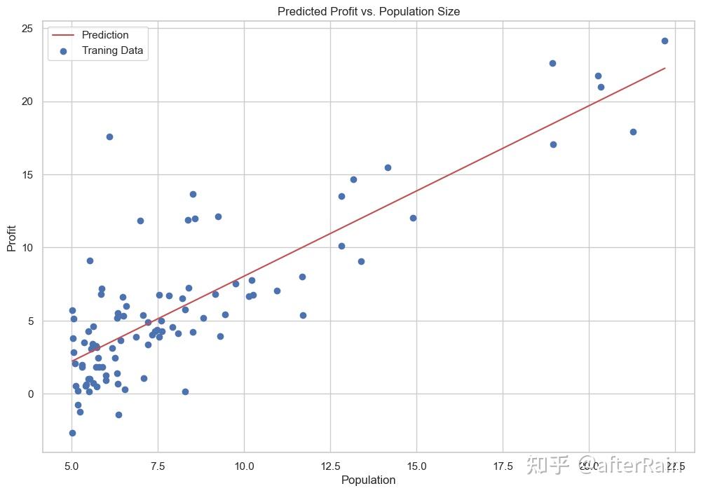
Linear Regression Visualize
1
2
3
4
5
6
7
8
9
10
11
12
| x = np.linspace(df.人口.min(),df.人口.max(),100)
f = g[0,0] + (g[0,1] * x)
fig, ax = plt.subplots(figsize=(12,8))
ax.plot(x, f, 'r', label='Prediction')
ax.scatter(df.人口, df.利润, label='Traning Data')
ax.legend(loc=2)
ax.set_xlabel('Population')
ax.set_ylabel('Profit')
ax.set_title('Predicted Profit vs. Population Size')
plt.show()
|
1
2
3
4
5
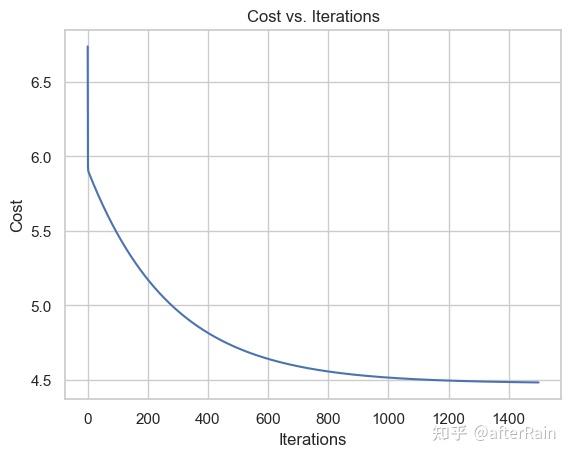
| sns.lineplot(x=np.arange(iters), y=cost)
plt.xlabel("Iterations")
plt.ylabel("Cost")
plt.title("Cost vs. Iterations")
plt.show()
|
Other Situation
1
2
3
| from sklearn import linear_model
model = linear_model.LinearRegression()
model.fit(np.asarray(X), np.asarray(y))
|
1
2
3
4
5
6
7
8
9
10
11
12
| x = np.array(X[:, 1].A1)
f = model.predict(np.asarray(X)).flatten()
fig, ax = plt.subplots(figsize=(12,8))
ax.plot(x, f, 'r', label='Prediction')
ax.scatter(df.人口, df.利润, label='Traning Data')
ax.legend(loc=2)
ax.set_xlabel('Population')
ax.set_ylabel('Profit')
ax.set_title('Predicted Profit vs. Population Size')
plt.show()
|
1
2
3
4
5
6
|
def normalEqn(X, y):
theta = np.linalg.inv(X.T@X)@X.T@y
return theta
final_theta2=normalEqn(X, y)
final_theta2
|

- 梯度下降:需要选择学习率α,需要多次迭代,当特征数量n大时也能较好适用,适用于各种类型的模型
- 正规方程:不需要选择学习率α,一次计算得出,需要计算,如果特征数量n较大则运算代价大,因为矩阵逆的计算时间复杂度为O(n3),通常来说当n小于10000 时还是可以接受的,只适用于线性模型,不适合逻辑回归模型等其他模型